There are No Straight Lines in Nature

Non-Linear Machine Learning

Antoni Gaudi was a Spanish Architect in the last 1800's where he said, "There are no straight lines or sharp corners in nature.  Therefore, buildings must have no straight lines or sharp corners"

If we agree with the premise that there are no straight lines in nature, it should also follow that with we should be careful with using linear machine learning models in practice.  There are certainly good use cases for Linear Models - but we have to be sure that the data in the range of we making predictions does in fact have a linear relationship.

However, the real world is messy and inherently non-linear.  How can we handle this case in Machine Learning.

In this post I will use a dataset of concentric circles, which are clearly non-linear, to show how linear  Scikit-Learn LogisticRegression fails, and then show how to use a Scikit-Learn RandomForest and a Tensorflow/Keras Neural Network to capture and predict using the non-linear data.

The goal of this article is see how to apply machine learning models to non-linear data.  It is out of scope to do a deep dive on any one particular model.

Here is a link to the Github Jupyter Notebook.  This article will talk to the highlights from the Jupyter notebook.

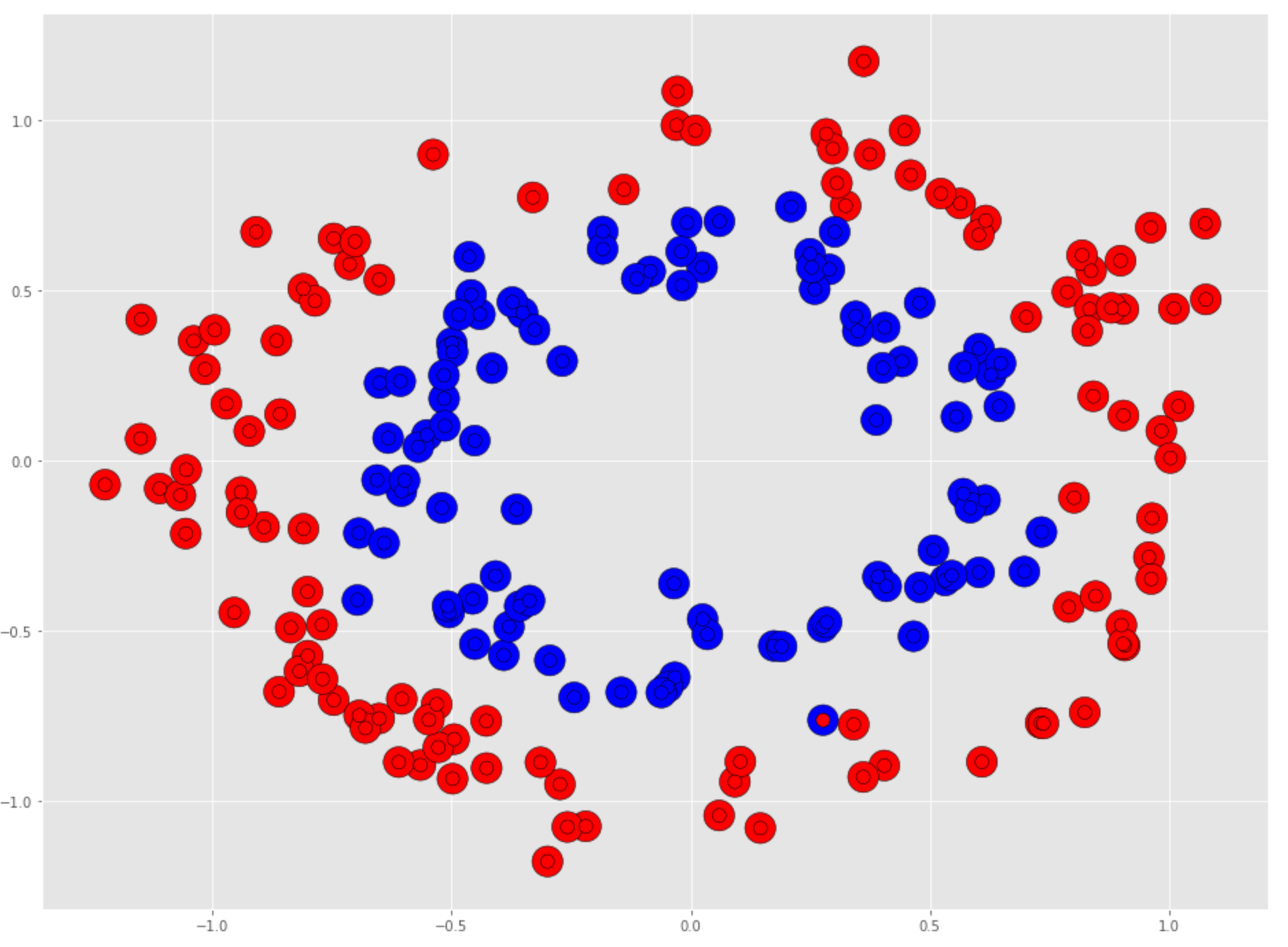
Circle Dataset

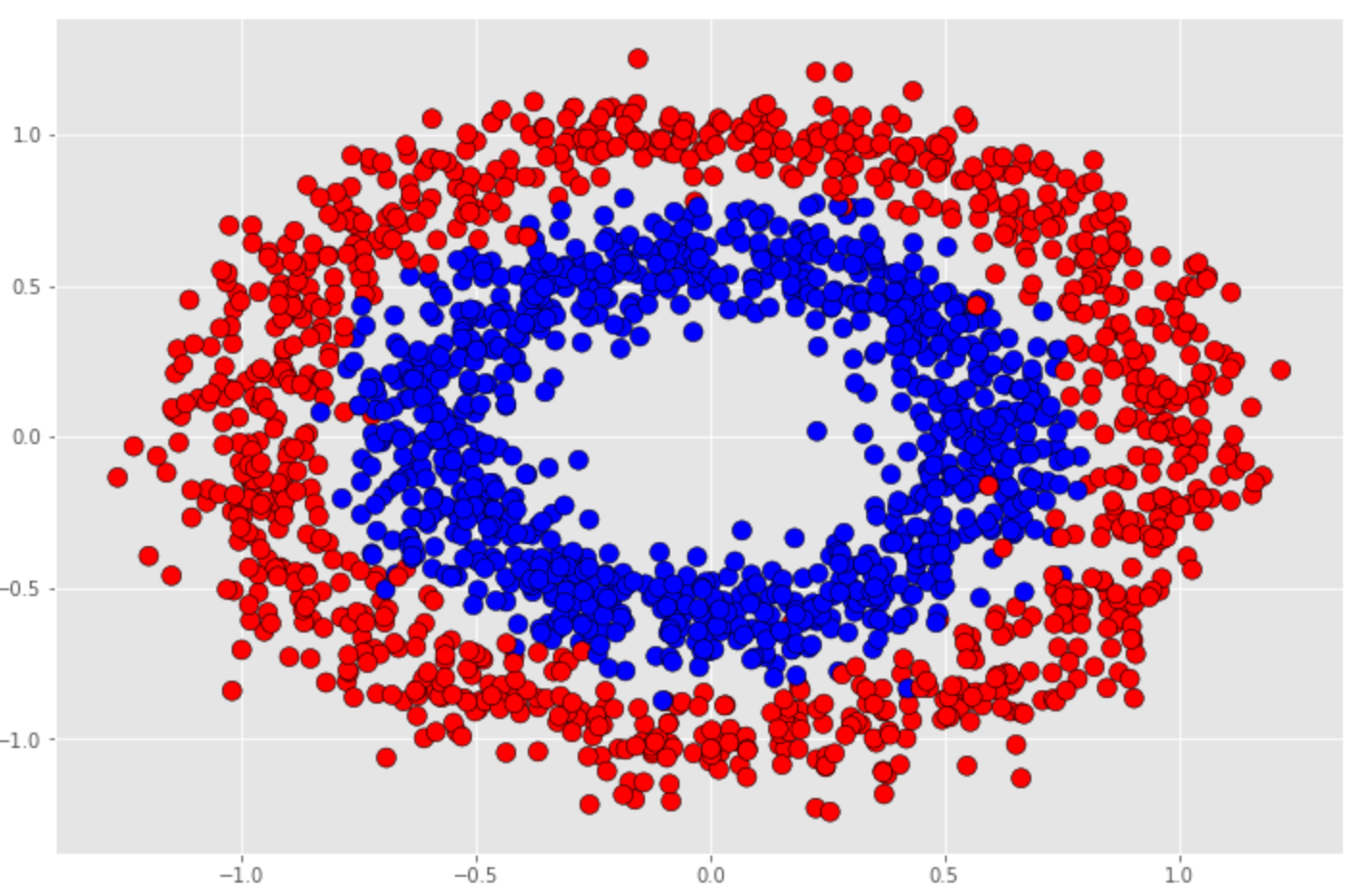
We will use this dataset to train models to make predictions to see how each model captures the non-linearity of the data.

Dependencies

This article assumes that all dependencies have been install on your local machine or you are using a hosted environment such as AWS SageMaker.

You will need to include:

• Python 3.6/3.7
• SciKit-Learn
• TensorFlow 2.x
• numpy
• pandas
• matplotlib

Setup

This article will assume all of the necessary components

Import the necessary libraries.  We are using sklearn ( SciKit-Learn ), Tensorflow and Keras.  Notice that this example assumes Tensorflow 2.0 with Keras included.

from sklearn.datasets import make_circles
from sklearn.model_selection import train_test_split

from tensorflow.keras.models import Model, Sequential
from tensorflow.keras.layers import Dense
from tensorflow.keras.optimizers import SGD

import numpy as np
import matplotlib
import matplotlib.pyplot as plt
%matplotlib inline

Create the circles dataset

Sklearn has a very convenient helper function for creating the circle dataset called, make_circles.

X, y = make_circles(n_samples=2000, factor=0.6, noise=0.1)

• Factor - scale factor between the inner and outer circle
• Noise - Standard deviation of Gaussian noise added to the data

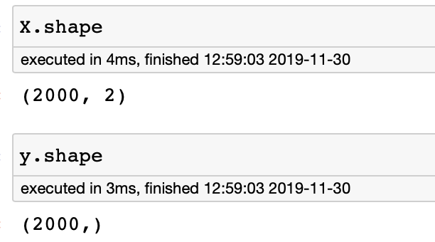
Look at the shape of the dataset to make sure it is what we expect.

Create Training, Testing, Holdout datasets

At a minimum we must divide our dataset into a training and testing dataset.  You never want to test your model on data that it used for training.  Many times you also want to create a holdout set, because the training and testing can be used during model train to verify accuracy, but the holdout is only ever used to test the generalization accuracy of a model.

Using a training, testing and holdout starts to be more important when you perform deep learning as we will see later.

Create a holdout dataset of 10% of the data, a testing dataset of 25% and a training dataset of 90% of the remaining total dataset.

X, X_holdout, y, y_holdout = train_test_split(X,y,test_size=0.1)
X_train, X_test, y_train, y_test = train_test_split(X,y,test_size=.25)

Linear Model - Logistic Regression

Let us try to apply a linear classifier to the circle data.  We do not expect this to do well, but it is instructive to see this and verify this outcome.

Instantiate a sklearn LogisticRegression Model

from sklearn.linear_model import LogisticRegression
logreg = LogisticRegression(solver='lbfgs')

logreg.fit(X_train, y_train)

Calling fit on the LogisticRegression model will use the training and testing data to determine the line of best fit.

We can see the coefficients and intercept calculated as below:

logreg.coef_ = array([[ 0.04117527, -0.07527537]])

logreg.intercept_= array([-0.00267699])

Score the model

View the testing and holdout dataset accuracy by calling score on the model.

logreg.score(X_test, y_test) = 0.48

logreg.score(X_holdout, y_holdout) = 0.45

As expected using a linear model to predict on non-linear data did not do well - in fact its worse than just guessing.

View holdout dataset performance

Lets look at how the holdout set performed by plotting the actual targets values overlayed with the predicted values.  Any red circle with a blue center, or a blue circle with a red center is where the prediction was incorrect.

Make predictions using the holdout dataset.

logreg_preds = logreg.predict(X_holdout)

Below is the code to plot the figure.

plt.figure(figsize=(16,12))

plt.scatter(X_holdout[:, 0], X_holdout[:,1], c=y_holdout, marker='o', edgecolor='k', s=500, cmap=binary_cmap)
plt.scatter(X_holdout[:, 0], X_holdout[:,1], c=logreg_preds, marker='o', edgecolor='k', s=100, cmap=binary_cmap)

line_bias = logreg.intercept_
line_w = logreg.coef_.T
points_x = np.linspace(-1,1,100)

points_y=[(line_w[0]*x+line_bias)/(-1*line_w[1]) for x in points_x]
plt.plot(points_x, points_y)

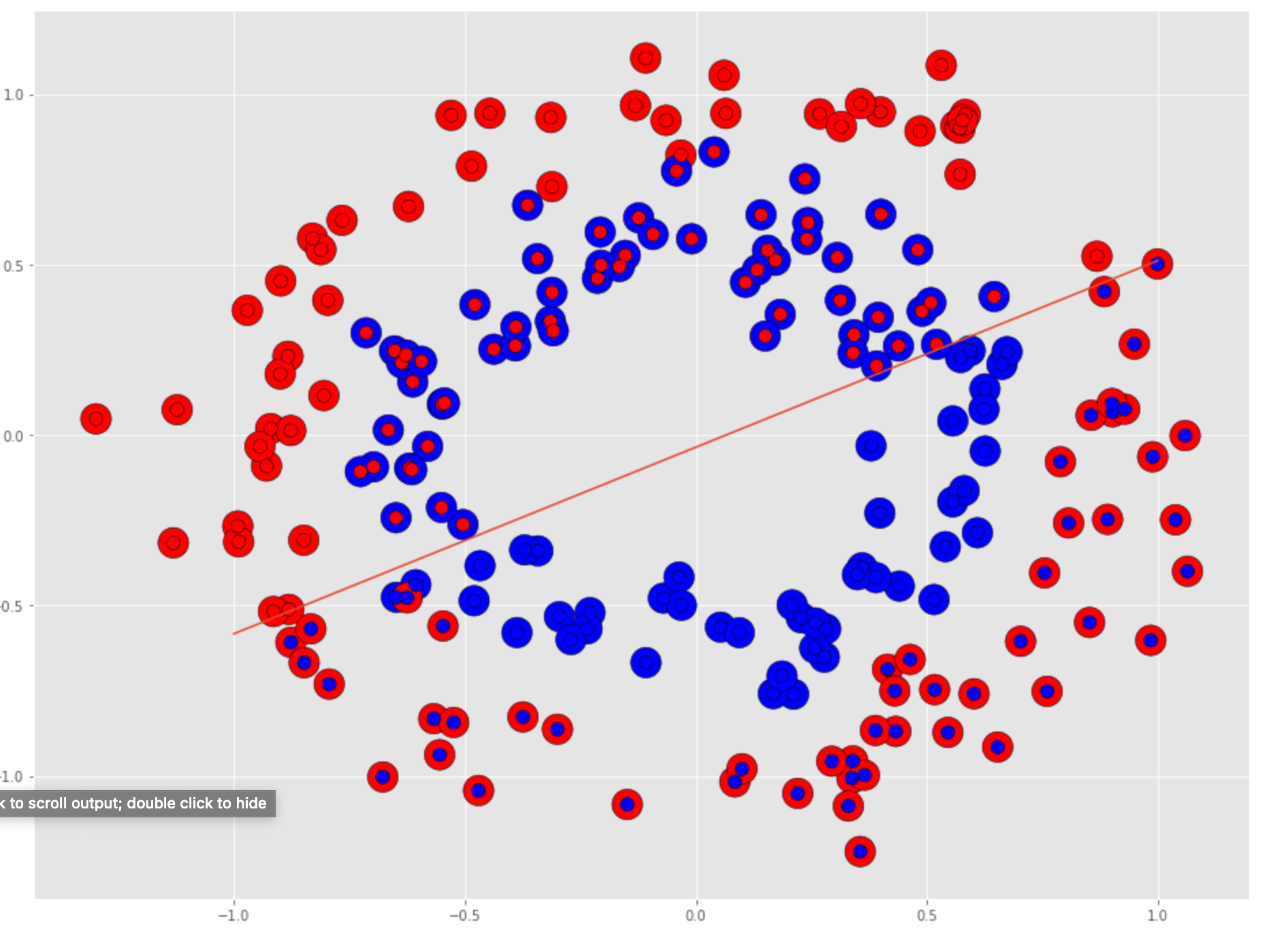
Visually we can see that we the LogisticRegression model had to split the holdout set into two halves which would only produce about a 50% accuracy.

How do you address this?  Use non-linear models.  We will look at 2 different models; a RandomForest machine learning model and a Tensorflow/Keras Deep Learning Neural network.

Non-Linear RandomForest Decision Tree

The SciKit-Learn RandomForestClassifier is an ensemble machine learning model made up of many  decision tree models.  A Decision Tree is a non-linear model built by constructing many linear boundaries.

RandomForest Model

Much like the LogisticRegression model, Scikit-Learn estimators follow a similar API.

from sklearn.ensemble import RandomForestClassifier
random_clf = RandomForestClassifier(n_estimators=100, max_depth=2)
random_clf.fit(X_train, y_train)

Score the Model

random_clf.score(X_test, y_test) = 0.818

random_clf.score(X_holdout, y_holdout) = 0.825

We can already see that the RandomForest classifier is performing much better, as one would expect.

View holdout dataset performance

Make predictions with the holdout dataset.

y_random_pred = random_clf.predict(X_holdout)

Plot the performance.  For the RandomForest there is no dividing line.  The plot will show all the predictions that matched the actuals, and any errors will have mixed color circle.

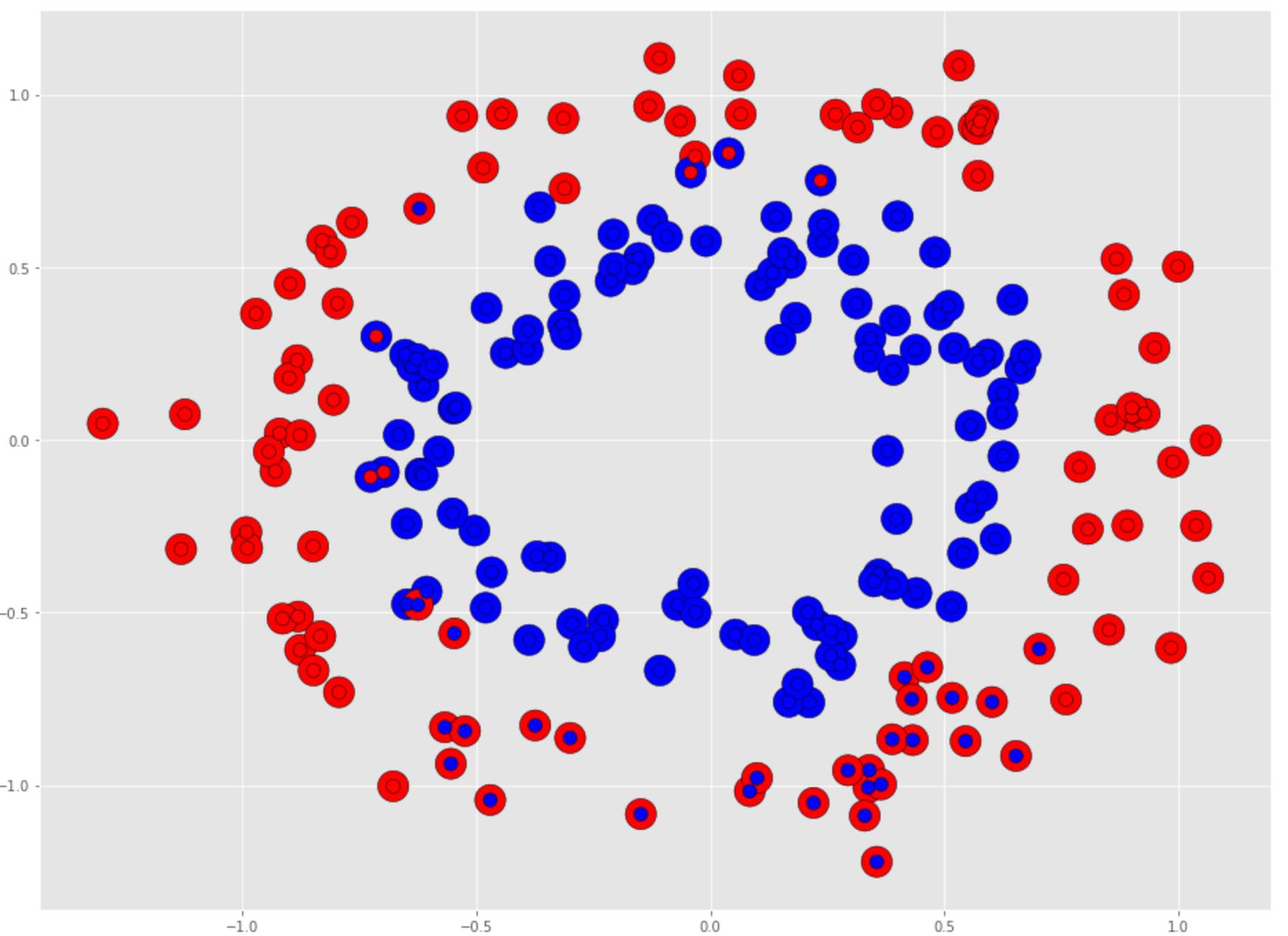
The RandomForest did much better, but there are still areas where the prediction struggled.  This model has not been tuned and it can likely be made to perform better.

Non-Linear TensorFlow/Keras Model

Next we will look at using TensorFlow with Keras to create a deep neural network - albeit not a very deep model, but one that performs well.

In this section we will explore Deep Neural Networks which are inherently designed to handle the non-linear nature of data.

Keras Neural Network

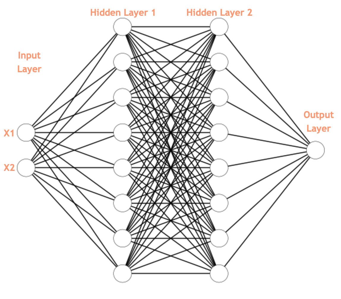
The neural network architecture will be a 2 input nodes, 8 hidden nodes, 8 hidden nodes, 1 output node.

The architecture would look like the following:

model = Sequential()
model.add(Dense(8, input_shape=(2,), activation="relu"))
model.add(Dense(8, activation="relu"))

model.add(Dense(1, activation="sigmoid"))
sgd = SGD(0.01)
model.compile(loss='binary_crossentropy', optimizer=sgd, metrics=['accuracy'])

50 Epochs

Lets start with 50 Epochs, which each Epoch trains on the entire dataset.

num_epochs = 50
H = model.fit(X_train, y_train, validation_data=(X_test, y_test), epochs=num_epochs, batch_size=64)

This is where the train, test and validation datasets really come into play. Notice we fit the model on the training data, and provide the test data as the validation set.  This way TensorFlow/Keras can use the test data to calculate the testing accuracy and loss.

When we evaluate the model after 50 Epochs we see the following:

model_eval = model.evaluate(X_holdout, y_holdout, verbose=0)
list(zip(model.metrics_names, model_eval))

[('loss', 0.6217296767234802), ('accuracy', 0.715)]

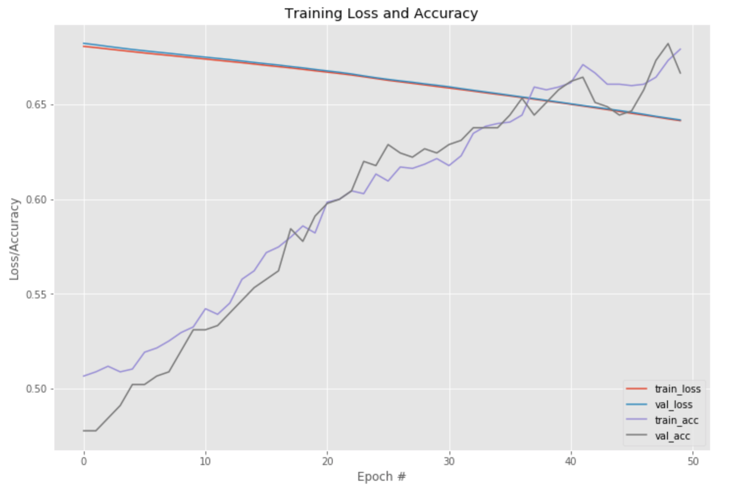
We can see that the model has yet to converge so we need to train with more Epochs.

600 Epochs

num_epochs = 600
H = model.fit(X_train, y_train, validation_data=(X_test, y_test), epochs=num_epochs, batch_size=64)

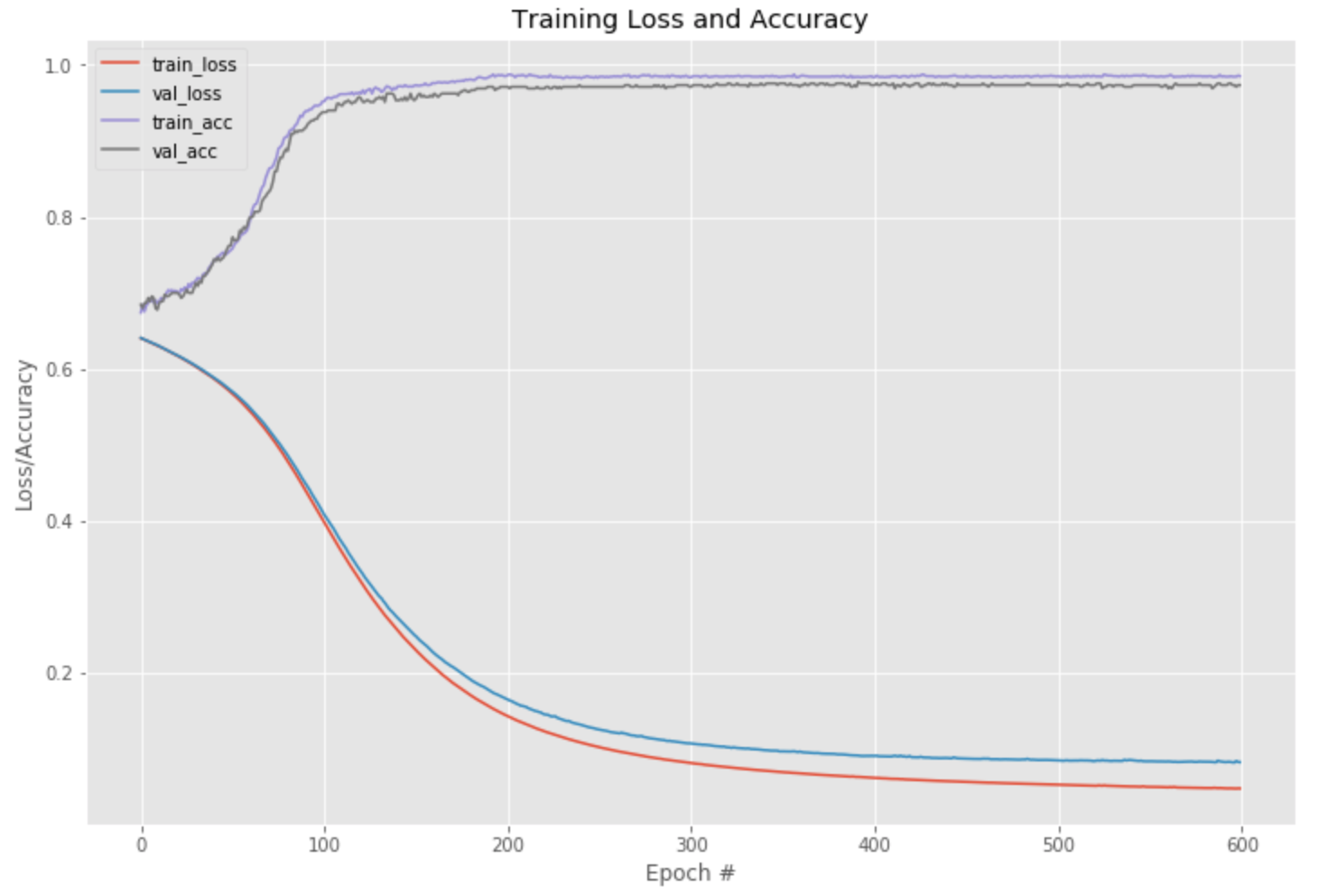
The Training Loss/Accuracy plot looks very good.  It shows that really after 200 Epochs the model did not improve, nor did it have a lot of room to improve.  We could have stopped the Epochs around 250 in this case.

View holdout dataset performance

We evaluate the model after 600 Epochs:

model_eval = model.evaluate(X_holdout, y_holdout, verbose=0)
list(zip(model.metrics_names, model_eval))

[('loss', 0.051138629019260404), ('accuracy', 0.995)]

Which has very good accuracy performance or  99.5%.  Notice that the Neural Network is not very complicated, nor is it very deep and yet it performs very well.

You can see from the holdout set there is one lone incorrectly predicted data point.

Summary

In this article we looked at how to address non-linear data in Machine Learning.  The world around us is inherently non-linear.  Even though we might be able to model linearity, that linearity might only hold for a certain range of values as as you get to the extremes of the values non-linearities start to present themselves.

Understanding how to apply non-linear models to data is important.  There are Machine Learning algorithms that are non-linear, such as Decision Trees or Deep Learning Neural Networks which are inherently non-linear.

I have been asked, "since Deep Learning can be applied to both Linear and Non-Linear data, and Deep Learning can solve problems that Machine Learning can solve, should I always use Deep Learning?"

My feeling is no.  You should start with Machine Learning techniques because they are simpler and depending upon your dataset, they could work very well.  There is a principle called, 'Occams Razor' which essentially states that the simplest explanation for a solution to a problem is likely the best solution.

Starting with Machine Learning techniques is almost always the simpler approach if it works.  You can always scale up to a Neural Network if needed, but you will need more data, CPU, GPU, etc to get really good results.